The Strongest Signal Is the One You Can't Have

2026-09-10 ai maths

TimesFM is Google Research’s pretrained time-series foundation model. You hand it a history and it extrapolates. There is no fit(), no training split, no coefficients, no API key and no cloud account — you download a 1.32 GB checkpoint and it runs on a laptop CPU.

Out of the box, though, it only looks at the series itself, and almost nothing in the real world moves for reasons contained entirely in its own history. Version 3.0, released in August 2026, fixed that with native covariates — extra channels handed to the model alongside the target, split into two kinds. That split is the interesting part, and it is what this lab measures.

Nearly every write-up of TimesFM so far demos it on a synthetic sine wave. This one points it at hourly PM2.5 in Milan — a real, messy, physically driven series — and runs a rolling-origin backtest to find out what the covariate support is actually worth.

The lab is here: lab-timesfm-pm25-covariates. It runs with docker compose up, needs no credentials, and after the one-time checkpoint download it runs offline.

The answer, measured over 90 daily forecast origins across one Po Valley winter, is that the covariate support is worth a great deal — from exactly one of the two kinds, and the less obvious one.

Milan in January

The Po Valley is a basin ringed by the Alps and the Apennines. In winter it forms temperature inversions: a lid of warm air settles over cold air, the mixing layer collapses, and the basin’s emissions accumulate for days until wind or rain clears them out.

That makes Milan’s PM2.5 genuinely exogenously driven. The thing being predicted responds to weather, not only to its own past — which is the precondition for covariates to be worth anything at all. If they never help anywhere, they should at least fail to help here.

One of the six weather variables is the inversion made numeric: boundary_layer_height is the depth of the layer pollutants get to mix into.

The data is one committed CSV — 9,504 hourly rows from 2025-08-01 to 2026-08-31, pulled from two keyless Open-Meteo endpoints and joined on an identical hour grid. PM2.5, NO₂ and CO come from CAMS; temperature, humidity, wind, precipitation, pressure and boundary layer height come from ERA5 reanalysis. Committing the snapshot is what makes the backtest deterministic and the whole lab runnable offline.

The backtest window is winter, because that is where the variance is. Measured on the snapshot, December through February runs a mean of 52.01 µg/m³ with a standard deviation of 24.77 and a peak of 135.70. The following summer is mean 10.62, sd 3.92, peak 28.50. Forecasting the summer series would be easy and uninformative — it barely moves.

The distinction that dominates real forecasting

TimesFM 3.0 splits covariates by what you can know at forecast time:

past_only_covariates — measured up to the origin and no further. You know yesterday’s NO₂. You do not know tomorrow’s.
past_future_covariates — known across the horizon too, because a forecast of them genuinely exists. Tomorrow’s weather qualifies.

That reads like an API detail. It is the entire problem. Here is Pearson correlation with PM2.5 across all 9,504 hours, with the only column that matters in production stapled on:

Variable	r	Knowable in advance?
`carbon_monoxide`	+0.923	✗
`nitrogen_dioxide`	+0.793	✗
`temperature_2m`	−0.654	✓
`relative_humidity_2m`	+0.572	✓
`boundary_layer_height`	−0.419	✓
`wind_speed_10m`	−0.347	✓
`surface_pressure`	+0.144	✓
`precipitation`	−0.097	✓

The two strongest correlates, by a distance, are exactly the two you cannot have. CO and NO₂ are near-proxies for PM2.5 because they share its sources — traffic and heating — and its dispersion physics. A model that could see tomorrow’s CO would be superb at this. Nobody can see tomorrow’s CO.

Everything below those two rows is weaker and forecastable. So the real question is whether weaker-but-available beats stronger-but-unavailable, and by how much.

One caveat the lab is careful about: correlation here is linear and contemporaneous, and says nothing about the lagged or nonlinear structure the model can actually exploit. Under a log1p transform the dispersion variables strengthen considerably — boundary layer height to −0.593, wind speed to −0.403 — which fits the physical picture that PM2.5 scales roughly inversely with mixing volume rather than linearly.

Six configurations, one thing different at a time

The comparison is an ablation, so the configurations are declared as data with exactly one axis of variation between them.

labs/lab-timesfm-pm25-covariates/src/app/eval/experiments.py:

UNKNOWABLE_POLLUTANTS = ("nitrogen_dioxide", "carbon_monoxide")


@dataclass(frozen=True)
class Experiment:
    """One row of the scoreboard."""

    name: str
    kind: str  # "naive" or "timesfm"
    blurb: str
    past_only: tuple[str, ...] = ()
    past_future: tuple[str, ...] = ()
    leaky: bool = False

Five of the six rows are the honest comparison:

EXPERIMENTS: tuple[Experiment, ...] = (
    Experiment(
        name="seasonal-naive",
        kind="naive",
        blurb="Same hour yesterday. No model, no data beyond the target.",
    ),
    Experiment(
        name="timesfm-univariate",
        kind="timesfm",
        blurb="TimesFM on the PM2.5 history alone.",
    ),
    Experiment(
        name="timesfm-past-only",
        kind="timesfm",
        blurb="Plus measured NO2 and CO up to the origin, and no further.",
        past_only=UNKNOWABLE_POLLUTANTS,
    ),
    Experiment(
        name="timesfm-past-future",
        kind="timesfm",
        blurb=(
            "Plus tomorrow's weather, measured rather than forecast. That is "
            "the best case for these covariates, not target leakage - a real "
            "forecast would carry error a measured value does not."
        ),
        past_future=config.WEATHER_VARIABLES,
    ),
    Experiment(
        name="timesfm-both",
        kind="timesfm",
        blurb="Past pollutants and future weather together.",
        past_only=UNKNOWABLE_POLLUTANTS,
        past_future=config.WEATHER_VARIABLES,
    ),
    # ...

The sixth cheats on purpose — more on that below.

There is nothing in there to inspect

Worth being blunt about this, because it trips up anyone arriving from classical regression: nothing in this lab estimates a parameter. No fit(), no coefficients, no train/validation split, no gradient step, no hyperparameter search. The 330M-parameter checkpoint is downloaded frozen and every configuration runs identical weights.

So “how much is wind worth?” cannot be answered by reading a weight off the model. Whatever weighting exists is internal to a pretrained transformer and is not exposed as anything readable. It is answered by ablation: run with and without a set of covariates, change nothing else, and measure the difference in error.

That is what the scoreboard is, and it is why every configuration shares one context length, one horizon and one set of origins. An ablation only means something if exactly one thing differs.

The scoreboard has to be honest before it is interesting

A forecast error with no baseline is a number with no scale. The baseline here is nine lines and no model.

labs/lab-timesfm-pm25-covariates/src/app/forecast/baseline.py:

def seasonal_naive(frame: pd.DataFrame, built: Sequence[Window]) -> FloatArray:
    """Predicts each horizon hour with the same hour one day earlier."""
    series = frame[config.TARGET].to_numpy()
    predictions = []
    for window in built:
        origin = window.start + config.CONTEXT_HOURS
        start = origin - config.SEASONAL_PERIOD_HOURS
        predictions.append(series[start : start + config.HORIZON_HOURS])
    naive: FloatArray = np.stack(predictions).astype(np.float32)
    return naive

“Same hour yesterday” is harder to beat than it looks. Hourly PM2.5 has a strong 24-hour cycle driven by traffic and heating, so lagging the series by one day already reproduces most of its shape. On this window it scores MAE 17.83 µg/m³, and beating it is the one performance assertion the lab enforces. A zero-shot foundation model that cannot beat a one-line lag has no story.

The evaluation is rolling-origin: 90 daily origins at 00:00 UTC across the winter, each forecast independently from its own 512 hours of context.

labs/lab-timesfm-pm25-covariates/src/app/config.py:

# --- Backtest geometry. These exact values reproduce a seasonal-naive
# --- MAE of 17.83 ug/m3; changing them changes that number.
BACKTEST_START = "2025-12-01"
BACKTEST_END = "2026-02-28"
EXPECTED_ORIGINS = 90
CONTEXT_HOURS = 512
HORIZON_HOURS = 24
SEASONAL_PERIOD_HOURS = 24

That comment is not decoration. Reproducing the 17.83 baseline is what pinned the geometry in the first place: origins at 00:00 UTC on every day from 2025-12-01 through 2026-02-28 inclusive is exactly 90 origins, and no other reading of “90 daily origins across December to February” produces that number.

Ninety origins rather than one train/test split is the difference between one sample of forecast skill and an average over episodes, calm spells, weekends and holidays. Nothing is refit between them — there is nothing to refit.

The geometry is enforced rather than assumed, so a silently truncated window cannot slip into the scoreboard:

labs/lab-timesfm-pm25-covariates/src/app/forecast/windows.py:

def build_windows(frame: pd.DataFrame) -> list[Window]:
    """Turns origin timestamps into positional windows over `frame`."""
    positions = {stamp: i for i, stamp in enumerate(frame.index)}
    built: list[Window] = []
    for origin in origin_timestamps():
        if origin not in positions:
            raise WindowError(f"origin {origin} is not in the snapshot")
        start = positions[origin] - config.CONTEXT_HOURS
        end = positions[origin] + config.HORIZON_HOURS
        if start < 0 or end > len(frame):
            raise WindowError(f"origin {origin} does not have room for its window")
        built.append(Window(origin=origin, start=start))
    return built

The control that cheats on purpose

The sixth configuration is handed tomorrow’s NO₂ and CO as though they were forecastable:

    # ...
    Experiment(
        name="leaky-control",
        kind="timesfm",
        blurb=(
            "CHEATS. Hands the model tomorrow's NO2 and CO as if they were "
            "forecastable. Nobody can run this for real - it is here to show "
            "what target leakage looks like on a scoreboard."
        ),
        past_future=UNKNOWABLE_POLLUTANTS,
        leaky=True,
    ),
)

Its MAE is 6.39, far ahead of every honest configuration, and it is not a result. It is what target leakage looks like on a scoreboard, included so a reader can recognise the shape of it in their own benchmark — a number that is suspiciously, beautifully good because the model is being told most of the answer.

It also earns its keep as a wiring test, and the assertion is written to say so:

labs/lab-timesfm-pm25-covariates/src/app/eval/checks.py:

def _leakage_is_visible(results: dict[str, ExperimentResult]) -> CheckResult:
    leaky_mae = results["leaky-control"].scores.mae
    honest = {name: results[name].scores.mae for name in HONEST_TIMESFM}
    best_honest = min(honest.values())
    passed = leaky_mae < best_honest
    return CheckResult(
        "leakage-is-visible",
        passed,
        f"leaky-control MAE {leaky_mae:.2f} vs best honest {best_honest:.2f} "
        "ug/m3 - if this fails, the covariate arguments are being ignored",
    )

If the cheating configuration did not win, the covariate arguments would not be reaching the model at all, and every other row in the table would be meaningless. Leakage being visible is the structural proof that the harness is wired up.

Which leaves the thing that is deliberately absent from the check list, and the file says it out loud:

"""The assertions that decide whether this run means anything.

Note what is NOT here: whether the honest covariate configurations beat the
univariate one. That is the question the lab is asking, and asserting an answer
to it would make the answer worthless. It is reported, not enforced.
"""

Six hard checks gate the run — snapshot integrity, output shapes and finiteness, beating the baseline, leakage being visible, calibration sanity, and bit-identical determinism across two runs. Whether the covariates help is not one of them, and cannot be, because that is the question.

Two things the API does that no write-up mentions

Both of these were read out of the installed timesfm==3.0.1 wheel rather than trusted from prose, because 3.0 is newer than most people’s mental model of the library — including, emphatically, an LLM’s.

A 24-hour horizon is not a 24-hour horizon. TimesFM decodes in patches of 64 steps, and the requested horizon is rounded up to output_patch_length internally. Past-future covariates are then expected to span context + 64. Supply context + 24 with the default padding_mode="none" and you get a shape mismatch.

The fix is padding_mode="edge", which repeats the last known value across the 40-hour gap. The alternative — actually supplying 64 hours of weather — would mean claiming to know nearly three days ahead when the entire premise is a one-day forecast. Edge padding costs a flat covariate tail that the model partially ignores, and keeps the claim honest.

TimesFM3Evaluator is the wrong class here, even though it is what the package README demos. It hard-enforces padding_mode="none", which is incompatible with the point above, and it defaults use_symmetric_averaging to True, which runs the context in both directions and doubles the forward passes. On CPU that is the difference between a lab that finishes in a minute and one that does not.

So the call is TimesFM3Forecaster with every flag explicit.

labs/lab-timesfm-pm25-covariates/src/app/forecast/model.py:

        outputs = list(
            model.predict_batch(
                contexts=contexts,
                horizon=config.HORIZON_HOURS,
                past_only_covariates=(past_only_list if experiment.past_only else None),
                past_future_covariates=(
                    past_future_list if experiment.past_future else None
                ),
                return_quantiles=True,
                use_symmetric_averaging=False,
                make_positive=True,
                sort_quantiles=True,
                # horizon 24 rounds up to the model's 64-step output patch;
                # edge-pad the covariates over the difference rather than
                # pretending to know 64 hours of weather.
                padding_mode="edge",
            )
        )
        points = np.stack([out.forecast for out in outputs]).astype(np.float32)
        quantiles = np.stack([out.quantiles for out in outputs]).astype(np.float32)

Every flag there is load-bearing:

All 90 origins go in one call. predict_batch chunks them internally by per_core_batch_size, which is 8 here. Looping one origin at a time would pay the per-call overhead ninety times.
make_positive=True clamps forecasts at zero. A negative PM2.5 concentration is physically impossible, and letting one through would corrupt the quantile band.
sort_quantiles=True enforces monotone quantiles. Without it a model can emit a 0.9 quantile below its 0.1 quantile — quantile crossing — which makes the coverage statistic meaningless.
use_symmetric_averaging=False halves the forward passes. It is a variance reduction traded away for CPU runtime, and the determinism check confirms the cheaper path is still bit-reproducible.

The leakage you commit by accident

A lab about leakage is an embarrassing place to leak, so this is the part that got the most care.

Covariates are z-scored per channel before the model sees them. Surface pressure sits near 1000 hPa while precipitation is usually 0.0; passed raw, the largest-magnitude channel dominates for reasons of units rather than physics. The subtle part is which hours the mean and standard deviation are computed over.

labs/lab-timesfm-pm25-covariates/src/app/forecast/scaling.py:

def standardize_channels(block: FloatArray, n_context: int) -> FloatArray:
    """Standardises each row of `block` using its first `n_context` values.

    `axis=1` with `keepdims=True` gives one mean and one standard deviation
    per channel, shaped (channels, 1), which broadcasts back across time.
    Using axis=0 would standardise across channels at each timestep - mixing
    pressure with rainfall - which is meaningless.

    The `_MIN_SD` floor keeps a channel that never moves inside its context
    from dividing by zero and seeding inf/nan through the whole forecast. It
    is defensive: across the 90 origins in this window the smallest context
    standard deviation of any channel is 0.043, so it never actually fires
    here.
    """
    context = block[:, :n_context]
    mean = context.mean(axis=1, keepdims=True)
    sd = np.maximum(context.std(axis=1, keepdims=True), _MIN_SD)
    scaled: FloatArray = ((block - mean) / sd).astype(np.float32)
    return scaled

block[:, :n_context] is the whole ballgame. A past-future covariate block extends one horizon past the origin, so computing its statistics over the full block would fold information about the future into the scaling of the inputs. The forecast would improve, and the improvement would be an artefact — the kind that never shows up as a failing test, only as a number that is quietly too good.

Two smaller things in the same nineteen lines. axis=1 with keepdims=True gives one statistic per channel; axis=0 would standardise across channels at each timestep, mixing pressure with rainfall, which is meaningless. And the _MIN_SD floor is documented as defensive rather than quietly relied upon: across all 90 origins the smallest context standard deviation of any channel is 0.043, because Milan gets enough winter rain that no 512-hour window is completely dry. An untested guard is a claim, not a safeguard.

The target itself is deliberately not standardised. It goes in as raw µg/m³, so forecasts and quantiles come back in the units of the problem and there is no inverse transform for a bug to hide in.

One more shape detail, of the sort that would not raise if you got it wrong:

def target_context(frame: pd.DataFrame, window: Window) -> FloatArray:
    """The target's context as a 1-D array.

    TimesFM keys its output shape off the input rank: a 1-D context yields
    (horizon,) and (horizon, 9). Keeping this 1-D is what gives the lab its
    (24, 9) quantile blocks.
    """
    context: FloatArray = context_block(frame, window, [config.TARGET])[0]
    return context

A 1-D context of length 512 yields a (24,) forecast and (24, 9) quantiles. A 2-D (1, 512) context yields (1, 24) and (1, 24, 9) and quietly changes every downstream shape. The sibling context_block has the same flavour of hazard in its .T: transposing pandas’ (time, channels) into the (channels, time) layout the model expects is not optional, and getting it backwards does not error — it forecasts a transposed nonsense series.

What the covariates were actually worth

This is the run, verbatim:

Scoreboard (PM2.5, ug/m3, 24h ahead)
---------------------------------------------------------------
configuration              MAE    RMSE    MASE  coverage  notes
seasonal-naive           17.83   23.50   1.000         -  Same hour yesterday
timesfm-univariate       12.08   15.79   0.678      0.80  TimesFM on the PM2.5 history alone
timesfm-past-only        12.17   15.82   0.683      0.79  Plus measured NO2 and CO up to the origin, and no further
timesfm-past-future      10.14   13.02   0.569      0.81  Plus tomorrow's weather, measured rather than forecast
timesfm-both             10.28   13.16   0.577      0.81  Past pollutants and future weather together
leaky-control             6.39    8.53   0.359      0.81  CHEATS *

Zero-shot forecasting on its own is already the headline nobody should skip past: 12.08 against the baseline’s 17.83, a 32% error reduction, with no training, no tuning and no feature engineering, on a series the model has never been pointed at.

Then the covariates.

Tomorrow’s weather is worth about 16% of MAE — 12.08 down to 10.14, MASE 0.678 down to 0.569. That is the single biggest honest gain in the table.

Yesterday’s NO₂ and CO are worth nothing at all — 12.08 to 12.17, very slightly worse than using the PM2.5 history alone. Stack them on top of the weather and it costs a little more: 10.14 to 10.28 for timesfm-both.

So the +0.92 correlate is worth less than nothing, and the −0.35 correlate is part of what buys the 16%. “Most predictive” and “actually knowable” are different questions, and only the second one pays.

Two disciplined readings of that table before anyone quotes it:

The 0.09 gap is noise. With 90 heavily overlapping, serially correlated origins there is no significance test here and ordinary confidence intervals do not apply. Nothing that small should be read as a finding. The 1.94 gap to timesfm-past-future is large enough to read as real.
The MASE column is not textbook MASE. Hyndman & Koehler scale by the in-sample one-step naive error; this scales by the seasonal-naive error on the same evaluation origins, which makes it a relative MAE. Useful here, not comparable to a MASE quoted anywhere else, and the lab labels it as such.

There is a runtime footnote too. From the run log, the 90 origins take 4.1 seconds for timesfm-univariate, 10.0 for timesfm-past-only, 21.8 for timesfm-past-future and 28.1 for timesfm-both. The past-only covariates more than double the compute to deliver a result that is fractionally worse.

The upper bound nobody should skip

This is the caveat that matters most to anyone tempted to take 16% to their own roadmap.

The “tomorrow’s weather” fed to timesfm-past-future is ERA5 measured reanalysis for those exact hours — not a real 24-hour weather forecast. That is not target leakage; PM2.5 itself is never leaked to any honest configuration. But it is the best possible case for weather covariates. A genuine forecast carries error that a measured value does not, so a deployed system feeding TimesFM real forecast weather would see less than 16%.

Treat it as an upper bound on what the covariate support is worth here, not a number production would get. It is exactly the sort of figure that gets quoted without its asterisk.

Two more limits, stated because a scoreboard without them invites over-reading. TimesFM’s training cutoff is not published, so a clean zero-shot result cannot be proven, only argued from the 2026 evaluation window — treat “zero-shot” here as a reasonable assumption rather than a demonstrated fact. And this is one city, one winter, one target; nothing here establishes that the result transfers to a coastal site where the inversion story does not apply.

The picture that is not flattering

The lab plots the worst episode in the backtest window rather than a good day.

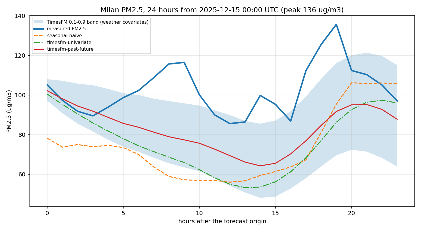
Origin 2025-12-15, peak 136 µg/m³. Every configuration badly underestimates it. The measured line spikes twice and the forecasts smooth straight through both. The 0.1–0.9 band — nominally 80%, and empirically 0.81 across the whole backtest — contains the truth for only 14 of these 24 hours, and never comes close to 136.

Two things survive in the mess, and together they are the lab’s result in one picture. The red line, with the weather covariates, sits above the green univariate one for the first 21 of the 24 hours: the weather told it not to let go of the smog as quickly. And the orange seasonal-naive line is the furthest-off of the three for the first half of the episode, which is the baseline earning its place on the chart. Even on the model’s worst day the ordering holds — episode MAE 29.3 for seasonal-naive, 26.5 for univariate, 20.1 with the weather.

A cherry-picked good day would have told you far less about whether to trust this on your own data than the model’s actual worst showing does.

What to take from it

If you are deciding whether any of this belongs in your own pipeline, three things:

Zero-shot foundation forecasting is real. A 32% error reduction over seasonal-naive, on a messy physical series, for the cost of a pip install and a 1.32 GB download. No GPU. No key. That was not true two years ago.

Covariates are worth plumbing in only if you can genuinely know them at forecast time. This is the part you cannot get from a correlation matrix, and it is why the two-kind split in the API is a modelling decision rather than a signature detail. Your strongest predictor may be worth nothing — worse than nothing, once you have paid for the compute to feed it in.

Build the boring baseline before you believe any of it. Seasonal-naive took nine lines here and it is still beating a 330M-parameter transformer for the first hour of every forecast. Without it, 10.14 µg/m³ is a number with no scale, and the leaky control’s 6.39 looks like a triumph.

Before you build on it

The TimesFM 3.0 model weights are licensed under timesfm-non-commercial-license-v1.0 — non-commercial, non-production use only. Anything built against those weights inherits that restriction. The TimesFM source code and the weights up to version 2.5 are Apache-2.0; if you need commercial use, the route is TimesFM 2.5’s weights plus its XReg covariate wrapper, not 3.0.

Data is © Open-Meteo, licensed CC-BY-4.0; air quality from the Copernicus Atmosphere Monitoring Service, weather from ERA5 reanalysis.

The lab is lab-timesfm-pm25-covariates. docker compose up runs the whole thing; a cold run from a fresh clone took 2:14 including the checkpoint download, and every run after that is offline and takes a bit over a minute on a laptop CPU. Its docs/METHOD.md carries the full method — every preprocessing step, the metric formulas, and a threats-to-validity section that is longer than it is comfortable to write.