Three Valleys, One Gradient Step
Picture a ball on a landscape with three valleys. A rule that always moves downhill will find a valley, but which one depends on where the ball starts. Gradient descent has the same limitation when its cost function has several local minima. In one dimension, we can see every move rather than hiding it inside a large model.
The lab
runs the same 100-update loop from x = -2.6, 0.5, and 2.6. It writes a
two-panel plot and complete CSV and Markdown tables. The function, derivative,
starting points, and learning rate are fixed, so the paths can be reproduced
with docker compose up --build from the lab directory. No account or external
data is needed.
A cost with three valleys
The cost is f(x) = x²(x² − 4)² / 16 + x / 10. The squared factors give the
curve several low regions; the x / 10 term tilts them so they do not all have
the same depth. Expanding gives x⁶/16 − x⁴/2 + x² + x/10.
Differentiating term by term gives
f′(x) = 3x⁵/8 − 2x³ + 2x + 1/10, or, in factored form,
x(x² − 4)(3x² − 4)/8 + 1/10. The lab evaluates that known slope directly:
labs/lab-gradient-descent-1d/src/app/experiment.py:
def derivative(x: float) -> float:
    """Evaluate the analytical derivative at a finite point."""
    if not _is_finite_real(x):
        raise ExperimentError(f"x must be finite, got {x}")
    value = x * (x * x - 4) * (3 * x * x - 4) / 8 + 0.1
    if not math.isfinite(value):
        raise ExperimentError(f"derivative is non-finite at x={x}")
    return value
The derivative tells us the direction of the local slope. At a point with a
positive slope, subtracting it moves x left; a negative slope moves x
right. With learning rate 0.04, each update is
x_next = x − 0.04 × f′(x). The rate controls the size of each move, while
the derivative supplies its direction and scale.
One row tells you the next
The loop records the current position, cost, and slope before each update.
That matters when reading the table: the slope in row k determines the
position in row k + 1.
labs/lab-gradient-descent-1d/src/app/experiment.py:
        for iteration in range(steps + 1):
            row = _record_state(run, iteration, x)
            rows.append(row)
            if iteration < steps:
                x -= learning_rate * row.slope
Here are the first four rows of the left run, copied from the lab’s
generated output/iterations.md:
| run | iteration | x | cost | slope |
|---|---|---|---|---|
| left | 0 | -2.6 | 2.9584360000000016 | -14.503160000000005 |
| left | 1 | -2.0198736 | -0.200359915125112 | -0.06620070631879924 |
| left | 2 | -2.017225571747248 | -0.20050472154481033 | -0.0432123158076641 |
| left | 3 | -2.0154970791149416 | -0.200566551326031 | -0.02834810285373976 |
At iteration 0, the slope is about -14.50316. Substituting it into the
update gives -2.6 − 0.04 × (-14.50316) = -2.0198736, exactly the next
row’s position. The next slope is much smaller, so the following move is only
about 0.002648. The left path has already reached the neighborhood of its
valley after one large step; the remaining updates refine its position.
Each run records iterations 0 through 100, so the two tables each contain
303 data rows. Start with the readable output/iterations.md; use
output/iterations.csv when you want the full values for your own checks.
Three starts, three endings
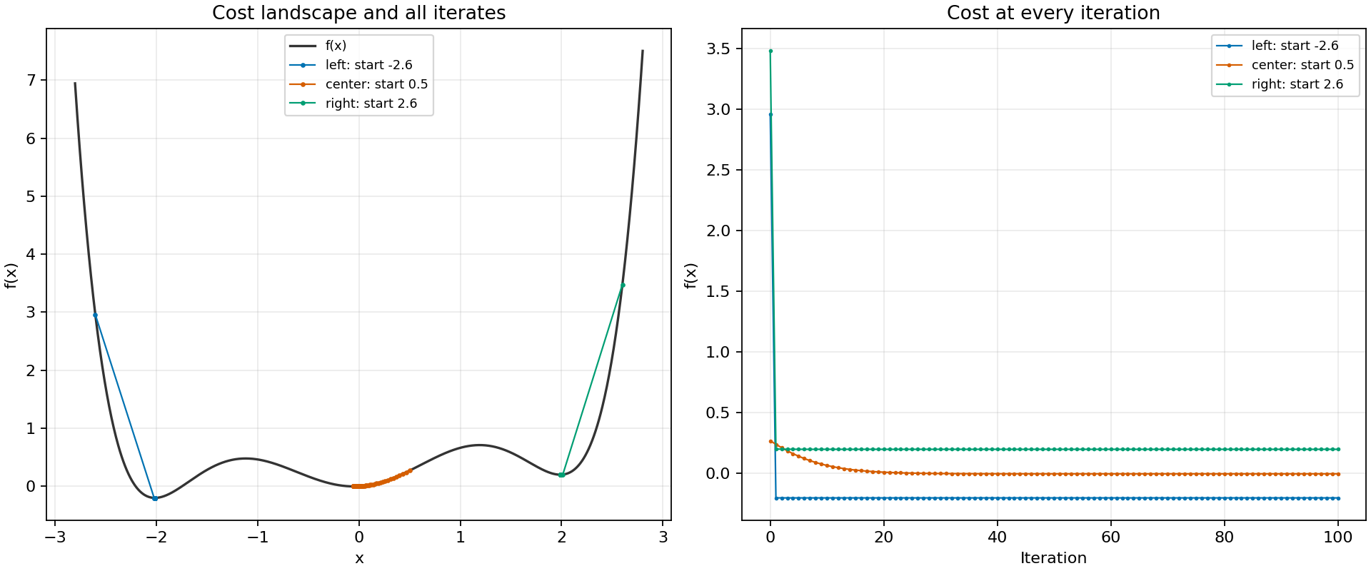
The left panel draws every recorded position on the cost curve. Many late points overlap where a path settles. The right panel uses iteration on the horizontal axis, so those later steps remain visible even when the position barely changes.
After 100 updates, the left run reaches approximately x = -2.012164 with
cost -0.200614. The center run reaches x = -0.049972 with cost
-0.002503; the right run reaches x = 1.987131 with cost 0.199363.
The left start found the lowest observed result of the three. Starting in
the center or right basin did not carry the same update rule across the hill
to the left valley.
These endings are not merely a plotting effect. The lab records all three paths through one call pattern:
labs/lab-gradient-descent-1d/src/app/commands/run.py:
        rows = tuple(
            row
            for name, start in (("left", -2.6), ("center", 0.5), ("right", 2.6))
            for row in gradient_descent(start, 0.04, 100, run=name, log=log)
        )
Only the start changes. Each run uses the same derivative, learning rate, and number of updates.
What the comparison proves
Trying several starts is useful: it finds a better result here than either the center or right run alone. It does not, by itself, prove that no lower valley exists elsewhere. Finite gradient descent runs also approach a minimum numerically; they do not reach an exact stationary point by declaration.
For this particular polynomial, there is a separate global-minimum
argument. Its derivative has five real stationary points: three local minima
near -2.012, -0.050, and 1.987, separated by two local maxima. A
degree-five derivative can have no more than five real roots, and the positive
x⁶ leading term sends the cost to positive infinity as |x| grows. Comparing
the costs at those three minima identifies the left one as the global minimum
of this function. That mathematical check supports the example; multi-start
gradient descent has no general global-optimum guarantee for nonconvex costs.
One dimension makes the update easy to inspect: one number, one analytic slope, one recorded move at a time. A later lab can extend the same idea to multiple parameters and a numerically estimated derivative, where the path is harder to picture but the question of where a start leads remains.
Run the complete lab to inspect every table row and reproduce the plot.